What is MEG?

The word magnetoencephalography (MEG), roughly translated to magnetic brain recording, is a non-invasive, passive, and silent method that measures weak magnetic fields that occur as the result of brain activity. By measuring these magnetic fields at multiple locations around the head one can infer where in the brain the activity originates from.

Two people are sitting in front of a large TV screen. One person is sitting under a MEG scanner

MEG recordings at NatMEG in a conventional MEG scanner (from left to right Christoph Pfeiffer and Andreas Gerhardsson). Photo: Daniel Lundqvist

Signal origin

Neurons, the cells that form the basic processing unit of the brain, produce a weak electric current when activated. Just like any other current, this neural current generates a magnetic field that curls around the current direction according to the right-hand curl or grip rule, where the extended thumb of the right hand represents the current direction and the fingers “grabbing the current” show the direction of the magnetic field. Unlike electric fields, magnetic fields extend relatively undisturbed through the brain, skull, scalp and into the space surrounding the head. A single neuron does not produce strong enough magnetic fields to be measurable outside the head. The magnetic fields we measure in MEG are instead the summation of the magnetic fields generated by tens of thousands of aligned neurons that fire at approximately the same time. Due to this spatial and temporal summation, MEG is most sensitive to pyramidal cells in the cortex (which are roughly aligned perpendicular to the surface of the grey matter) and postsynaptic potentials (which last approximately 10x longer than action potentials). When measuring outside the head we are most sensitive to tangential sources, that is sources in the cortex that are oriented parallel to the head surface, and less sensitive radial sources, that is sources pointing out or into the head surface. One should keep in mind that the head is not a perfect sphere, and most sources neither entirely radial nor tangential.

How do we measure MEG?

Conventional MEG scanner

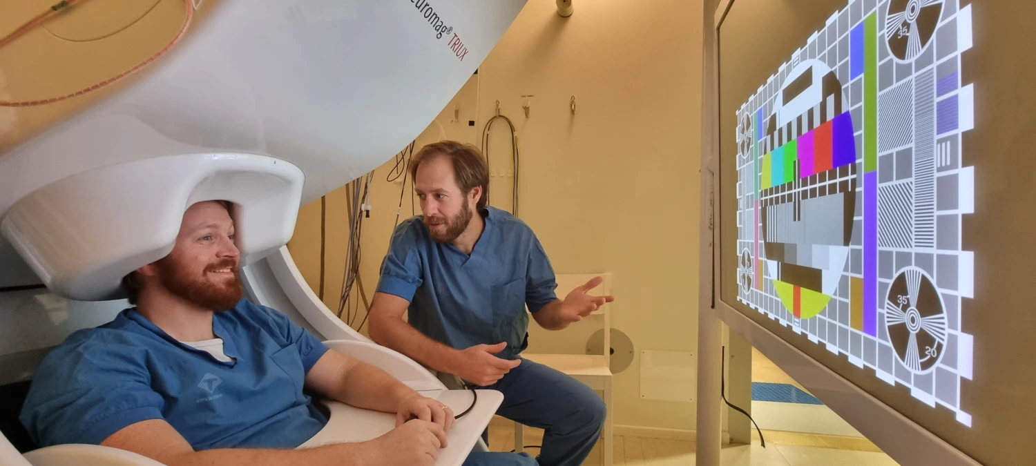
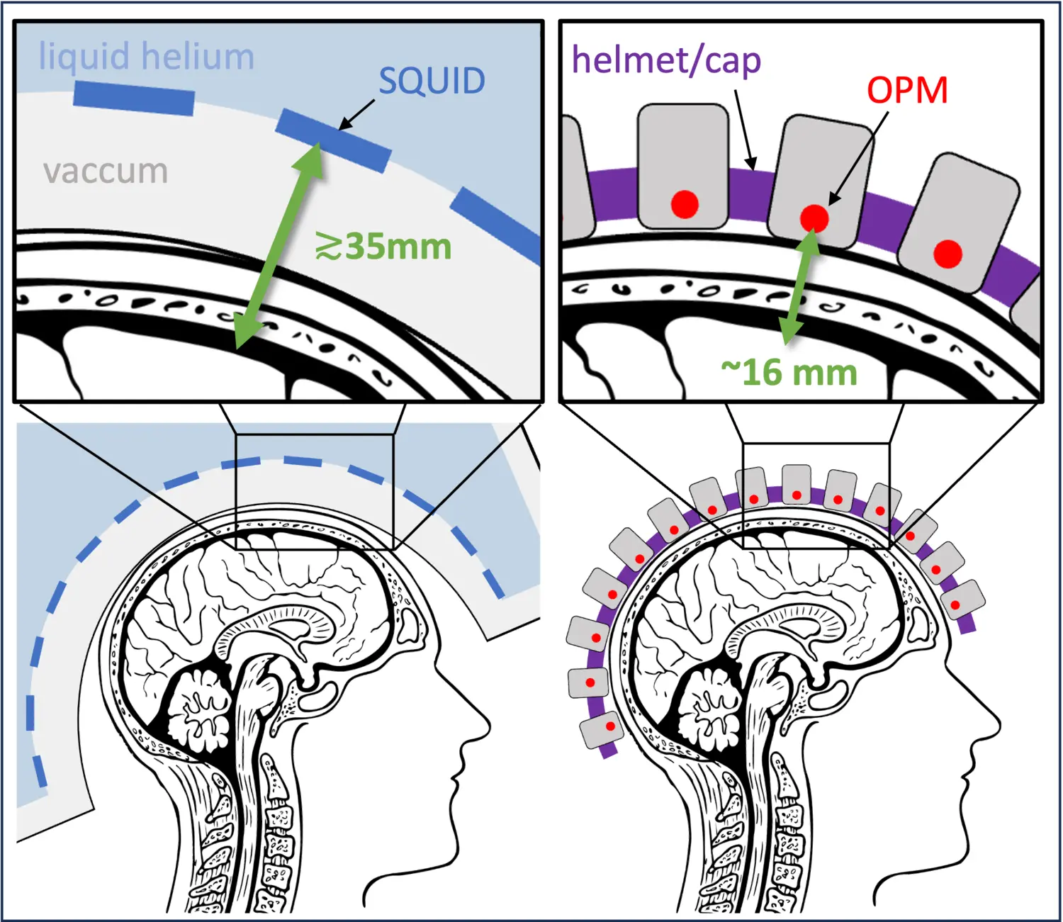
A typical MEG device consists of 100-300 highly sensitive sensors arranged around the subject’s head. Conventional MEG uses extremely sensitive magnetic field sensors, so-called superconducting quantum interference devices or SQUIDs. As the name suggests SQUIDs require superconductivity to work. Superconductivity is a quantum physical state where the material becomes a perfect electric conductor and expels magnetic fields. To date, superconductivity can only be achieved at cryogenic temperatures (and/or extreme pressures). Conventional SQUIDs must be cooled to less than ~9 K (~-265 °C). This is usually achieved with liquid helium (~4 K; ~-269 °C) and requires substantial thermal insulation between the cold sensors and the room temperature environment. The thermal insulation in a MEG device is achieved by a combination of superinsulating foil and ~2 centimeters of vacuum. The MEG sensors are housed inside a double walled flask, where the volume between the two walls is hermetically sealed and vacuum pumped (similar to a thermos bottle).

SQUID

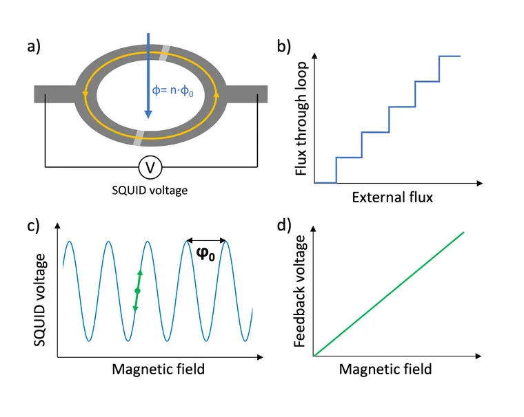
A SQUID consists of a superconducting loop with two weakly or non-superconducting links (Figure 2-a). Superconducting rings have the interesting property that they only permit flux in discreet steps through them – in other words the flux through a superconducting loop is quantized. If the externally applied field is larger or smaller than an integer multiple of the flux quantum, a current is induced that brings the total flux through the loop to the closest integer (Figure 2-b). Since superconductors exhibit zero resistance, these currents could normally not be measured. Here is where the weak links come in. Unlike in the superconductor, the current through a weak link generates a voltage that can be measured. Unfortunately, the induced voltage has a periodic relation with the magnetic field with the period equal to the flux quantum – which would severely limit the range in which the sensor can measure (Figure 2-c). To linearize the signal, a negative feedback loop is created with a small coil which counters any change in in the external magnetic field by generating an opposing field that keeps the SQUID voltage at a fixed point (called the working point; indicated by green dot in Figure 2-c). The current going to the feedback coil has a linear relation with the measured magnetic field and serves as the sensor output signal (Figure 2-d).

Figure 1: a) Schematic of a SQUID consisting of a superconducting ring (dark grey) with two weak links (light grey). Externally applied magentic field and induced current are indicated by blue and yellow arrows respectively. b) Flux quantization. c) SQUID voltage as a function of externally magnetic field. Working point of negative feedback scheme is Image: Christoph Pfeiffer

Pickup coils

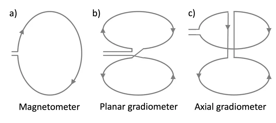
Pick-up coils (the large input coil of a flux transformer) come in different forms and shapes that affect how the combined sensor measures the magnetic field. They can be roughly divided into two categories. Simple loops create magnetometers - sensors whose output is proportional to the magnetic field through the loop. Double loops with opposing windings, such as a figure-8 coil, create gradiometers - sensors whose output is proportional to the difference between the magnetic fields through the different loops. In the figure-8 coil example, that would be the difference between top and bottom loop which would effectively result in measuring the vertical gradient of the magnetic field that is perpendicular to the plane (i.e., that points out of the page or screen). Higher order gradiometers can be achieved with more complex pick-up loop configurations.

The advantage of gradiometers lies in the fact that, while they are less sensitive than a magnetometer of the same size, they suppress external interferences. A faraway source, like a car driving by, will create an equal magnetic field in both loops and get cancelled out (assuming the two loops are the same and opposite wound), while a close source, such as neuronal activity will create different magnetic fields in the two loops. Typical MEG scanners use magnetometers and/or first-order gradiometers.

Figure 2: Example of pickup loops forming a magnetometer (a), planar (b) and axial gradiometer (c). Image: Christoph Pfeiffer

SQUIDs are usually very small, only some tens to hundreds of micro(10-6)meter, which is suboptimal for magnetic field sensitivity. To increase magnetic field sensitivity, SQUIDs can be connected to a flux transformer consisting of a larger (pick-up) coil connected to smaller (coupling) coil. A flux transformer can be imagined as a funnel, that picks up the magnetic field over a large area and concentrates it onto the small area of the SQUID loop. Flux transformers are typically also superconducting, often even integrated into the same chip as the SQUID. Together the flux transformer and SQUID form the MEG sensor.

Magnetically shielded room

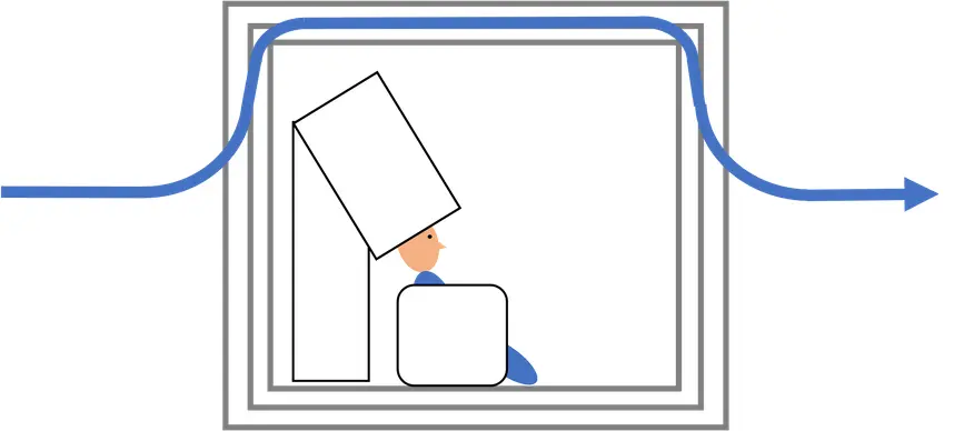
MEG scanners operate inside a magnetically shielded room, or MSR for short, that deflects most of the external magnetic interference from the environment that would otherwise mask the weak fields from the brain. For perspective, typical MEG fields are on the order of several tens to hundreds of femto(10-15)-tesla, roughly a hundred million to a billion times smaller than the earth’s magnetic field that is approximately 50 micro(10-6)-tesla. MSRs are constructed from multiple layers of high permeability metal, e.g., mu-metal, a ferromagnetic nickel-iron alloy, that deflect low frequency magnetic fields and high conductivity metal, e.g., copper, that shields high frequency magnetic fields. Some MSRs have additional active compensation where external fields are cancelled by generating opposing fields with coils, e.g., in the MSR walls.

Figure 3: Schematic of a magnetically shielded room housing a MEG scanner illustrating how the magnetic shielding (grey squares) diverts external magnetic fields (blue arrow). Image: Christoph Pfeiffer

What is on-scalp MEG?

Distance matters

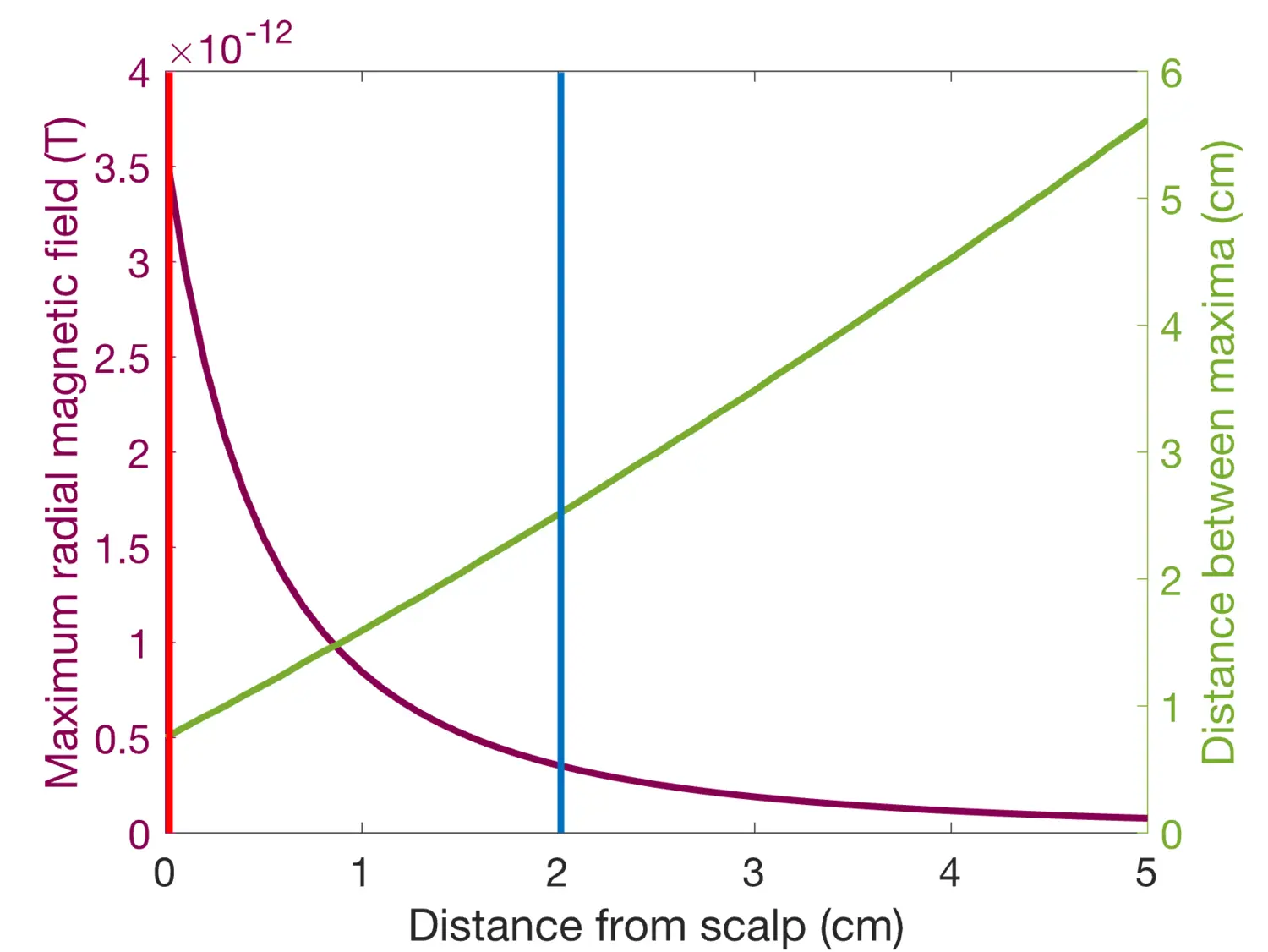
Magnetic fields quickly drop off with distance from their source (roughly following a one-over-distance-squared relation). As a result, MEG is generally more sensitive to shallow sources, that is sources close to the scalp - and therefore also clsoer to the sensors - than deep sources. Conversely, this means that sensors closer to the head pick up stronger signals from the same source than sensors further away. In addition to having higher amplitudes, the magnetic field patterns are more focal closer to the source, which makes it easier to distinguish nearby sources but requires denser sampling (i.e., packing the sensors more densely) to capture the all the minute details of the magnetic field distribution. As a result, measuring closer to the head, so-called on-scalp MEG (osMEG) systems, can achieve higher sensitivity and spatial precision than conventional MEG systems that measure at approximately 2 cm distance.

magnetic field generated by a single dipolar source as a function of distance

Figure 4: Strength (purple) and distance (green) between the peaks of the magnetic field generated by a single dipolar source as a function of distance. Red and blue vertical lines indicate the scalp and minimal distance when measureing with conventional MEG, respectively. Image: Christoph Pfeiffer

Sensors - OPMs

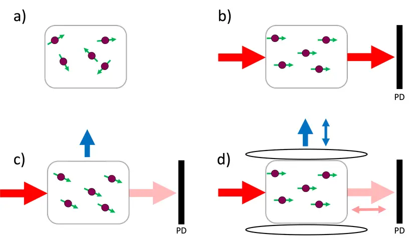
Optically pumped magnetometers (OPMs) are a highly sensitive type of quantum enhanced magnetic field sensors. At their heart OPMs have a glass cell filled with alkali metal vapor (most commonly rubidium or cesium). At rest the spins or angular moments of the alkali atoms are randomly oriented (Figure 2-a). By shining laser light of a specific wavelength into the vapor, the alkali atoms can be pumped into a state where their atomic spins are aligned (Figure 2-b). This involves the atoms absorbing some of the light. Once all the atoms are pumped into the aligned state, the vapor stops absorbing the laser light and becomes transparent to it. When a magnetic field is applied, e.g., perpendicular to the laser beam, the atomic spins start to precess around the magnetic field (Figure 2-c), similar to what happens in MRI. As the atomic spins start to precess, i.e., leave their aligned state, they begin absorbing the laser light again. This in turn drives them back towards the aligned state. Precession and laser light absorption balance each other, resulting in a reduction of the transmission through the vapor cell. The speed of the precession, and as a result the change in transmission, depends on the strength of the magnetic field (assuming the laser power is fixed). We can measure the transmission with a photodetector behind the vapor cell.

Figure 5: Schematic representation of an OPM. a) A vapor cell with rubidium atoms (purple) with randomly oriented spins (green arrows). b) Laser light (red arrows) shines into the cell and pumpes atoms into a state where all spins are aligned and do not absorb any more light. c) An external, transverse magnetic field (blue arrow) causes the atom spins to precess and absorb light. As a result less light reaches the photodiode (PD). d) A transverse, oscillating field is applied to the vapor cell using a Helmholtz coil. This results in a modulation of the transmitted light that can be detected at the photodiode and demodulated to obtain directional information. Image: Christoph Pfeiffer

There are a few important things to note here:

In contrast to SQUIDs, OPMs measure the absolute field.
The range is limited to low magnetic fields (typically few nT).
The direction of the magnetic field is unknown. We assumed a magnetic field direction perpendicular to the laser beam but any direction that is not exactly parallel to the laser beam would create a precession.

The unknown magnetic field direction can be solved with a set of coils (e.g., a Helmholtz coil pair) that generate an oscillating magnetic field in the vapor cell that is perpendicular to the laser beam (Figure 2-d). The oscillating magnetic field (typically ~1kHz) modulates the signal in the direction of the oscillating magnetic field. If we demodulate the signal from the photodiode, we get the signal in the direction of the oscillating magnetic field. The demodulated signal roughly corresponds to the gradient of the original resonance-like signal with a linear dependence on the magnetic field close to zero.

One of the main mechanisms limiting OPM sensitivity, the so-called spin exchange relaxation, can be overcome by increasing the alkali pressure inside the vapor cell. Sensors using this method are called spin exchange relaxation free (SERF) and achieve the lowest noise levels but have a limited measurement range. To achieve optimum alkali vapor pressure the vapor cell is often heated to around 160 °C. Suspending the vapor cell in a vacuum encapsulation for thermal insulation reduces the - already small - power consumption and minimizes heating the sensor surroundings.

The measurement range of a SERF OPM can be increased in a similar way to SQUIDs, by creating a negative feedback loop, where a coil generates a magnetic field that opposes the external magnetic field. The current through the coil that generates the opposing field serves then as the measurement signal. The magnetic field must be within the linear measurement range of the OPM when the negative feedback loop is activated. Alternatively, one must null the background field before engaging the feedback loop. This typically requires scanning the feedback magnetic field, since the background magnetic field is unknown.

Figure 6: Schematic representation of conventional MEG system using LTS SQUID sensors (left) compared to a on-scalp MEG system using OPM sensors (right). Image: Christoph Pfeiffer (head from public domain/CCO)

Even with a negative feedback loop, OPMs have a limited measurement range compared to SQUID sensors. Many magnetically shielded rooms (MSRs) that are perfectly suitable for conventional and HTS SQUID-based MEG systems do not offer sufficient shielding to operate OPMs reliably. Additional magnetic field nulling coils are used in these cases to further reduce the remaining magnetic field closer to the sensors.

A major advantage of OPMs in osMEG is their small size (a commercial SERF OPM sensor is roughly the size of a sugar cube) and weight (a few grams per sensor). This allows significantly more flexibility in designing sensor arrays compared to conventional MEG. A system only requires a light support structure that hold the sensors securely in place for the measurement. Such a support structure can be made from 3D-printed plastic, making it cheap and easy to prototype different sensor arrays with the same set of sensors. There are three main types of support structures for OPM-based on-scalp MEG. Helmets with depth-adjustable sensor slotswhere the sensors can be adjusted in one direction to fit the individual subject’s head size and shape, customized helmets, that are designed to perfectly fit a specific subject, and flexible caps similar to EEG caps that the sensors are attached to.

Fixing the support structure to the subject’s head (as in the case of a flexible cap) instead of to a chair or other large structure allows the subject to move their head, increasing subject comfort and enabling new types of experiments that were previously only possible with EEG. Moving the sensors however adds additional demands on the magnetic field compensation as movements in even a small magnetic fields create large artifacts.

Sensors – HTS SQUIDs

High temperature superconductors (HTS) are a group of materials that achieve superconductivity at significantly higher temperatures than conventional superconductors. Yttrium barium copper oxide (YBCO), for instance, becomes superconducting at ~92 K (~-180 °C). While this is still very cold it brings two major advantages: HTS SQUIDs can be cooled by liquid nitrogen (~77 K; ~-196 °C) – a much cheaper and more sustainable alternative to liquid helium – and the vacuum insulation can be decreased to as little as 1 mm. The latter makes HTS SQUIDs a great choice for osMEG. The higher temperature of HTS SQUIDs results in slightly higher noise, which is alleviated by the signal increase from coming closer to the head.

Since the working principle is the same as that of LTS SQUIDs used in conventional MEG, HTS SQUIDs have similar high bandwidth and dynamic range. While a HTS SQUID chip is very small (~10 mm x 10 mm x 1 mm) the necessary cryostat makes systems more a bit more bulky and less adaptable compared to OPM based osMEG systems.